Tidal and Current Modelling for Dredging and Pipeline Work

Dredging, pipeline installation, and nearshore construction all depend on water level and water motion. A dredge requires a known vertical reference to cut to design depth. A pipeline requires current loading estimates for on-bottom stability and installation analysis. A nearshore structure requires design water levels and current velocities that account for the combined effect of tide, wind, density, and waves. Tidal and current modelling provides these inputs, and its reliability depends on three connected elements: a defensible tidal datum, measured current data, and a hydrodynamic model that has been calibrated and validated against observations.

Tidal Physics and Harmonic Analysis

Tides are the response of the ocean to astronomical forcing, principally the gravitational attraction of the moon and sun combined with the centrifugal effect of the earth-moon-sun system's rotation. The forcing is periodic and predictable, which is why tides can be forecast with high skill at locations where sufficient observations exist.

The tide at a location is decomposed into harmonic constituents, each with a known astronomical frequency, an amplitude, and a phase that must be determined from observation. The dominant semidiurnal constituent is M2, with a period of approximately 12.42 hours. Other significant constituents include S2, N2, K1, and O1, which represent the solar semidiurnal, lunar elliptic, and diurnal components respectively.

Tidal harmonic analysis expresses the observed water level as h(t) = H₀ + Σ Aᵢ cos(ωᵢt − φᵢ), where H₀ is mean level, and Aᵢ, ωᵢ, and φᵢ are the amplitude, angular frequency, and phase of each constituent i. The accuracy of the resulting prediction depends on record length, data quality, and the stability of the local response.

The spring-neap cycle arises from the constructive and destructive interference of solar and lunar constituents and repeats approximately every 14.77 days. A longer modulation, the nodal cycle of about 18.6 years, affects the amplitude of certain constituents and is relevant to extreme water level statistics and to the definition of the lowest astronomical tide.

In the Arabian Gulf, tidal ranges are generally modest, typically in the range of one to two metres in many coastal locations, and the tidal regime varies from semidiurnal to mixed. This relatively small range does not reduce the importance of accurate tidal definition. In shallow water, small water level errors translate directly into dredge depth errors and into pipeline trench depth errors, and shallow-water tidal distortion produces asymmetric flood and ebb durations that a simple sinusoidal assumption will not capture.

Tidal Datum Definition and Vertical Reference

A tidal datum is a vertical reference defined by a particular phase or statistical level of the tide. Common tidal datums include:

• Mean sea level (MSL): The average water level over a defined period, commonly used as a national vertical reference.

• Mean high water springs (MHWS) and mean low water springs (MLWS): Statistical levels derived from spring tide predictions.

• Highest astronomical tide (HAT) and lowest astronomical tide (LAT): The extreme predicted levels under average meteorological conditions over the nodal cycle. LAT is widely used as chart datum because it ensures predicted water levels are almost always above the charted depth.

• Chart datum: The reference surface to which nautical chart depths and dredge design depths are reduced.

A chart datum defined at lowest astronomical tide ensures that charted depths are conservative, because actual water level will nearly always exceed the datum and therefore exceed the charted depth. Dredge design depths, trench depths, and pipeline cover requirements must be referenced to the same datum used in the design documents, and the transformation between chart datum, project datum, and ellipsoidal height must be documented explicitly.

The practical difficulty is that datums are local. A datum established at a reference port does not transfer directly to a construction site several kilometres away, because tidal amplitude and phase vary spatially. Datum transfer requires simultaneous observation at the reference gauge and the site, or a hydrodynamic model capable of resolving the spatial variation of tidal phase and amplitude. In shallow embayments, phase differences of tens of minutes between two nearby locations are common.

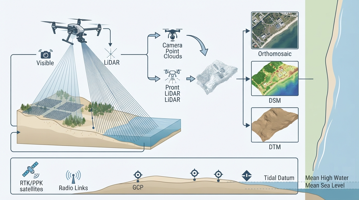
GNSS-derived ellipsoidal heights are increasingly used in marine construction, but they are referenced to an ellipsoid, not to a tidal datum. Converting between them requires a geoid model and a datum separation value that must be established from water level observation. Treating ellipsoidal height as equivalent to chart datum elevation is one of the most consequential errors in dredging and nearshore construction.

Currents and Their Forcing Mechanisms

Water motion in coastal and nearshore environments results from several superimposed forcing mechanisms, and design or operational decisions usually require the combined effect rather than any single component.

• Tidal currents: Oscillatory flow driven by the tidal pressure gradient, typically reversing in direction in channels and rotating in open coastal areas.

• Wind-driven currents: Surface and near-surface flow generated by wind stress, significant during sustained wind events.

• Density-driven currents: Flow generated by horizontal gradients in temperature and salinity, relevant in estuarine settings and in areas of high evaporation.

• Wave-induced currents: Near-bed orbital motion and longer-period currents such as longshore drift generated by wave breaking.

• Residual currents: The net non-oscillatory transport remaining after tidal averaging, which governs long-term sediment movement and plume advection.

In the Gulf, seasonal wind regimes, high evaporation, and restricted exchange with the open ocean produce density gradients and wind-driven circulation that can dominate the residual flow. Tidal currents in shallow channels may be strong even where the tidal range is modest, because the same water volume passes through a constricted cross-section. Local acceleration around dredged channels, reclamation edges, and berth pockets can produce velocities considerably higher than the ambient coastal flow.

Current Measurement Methods

Acoustic Doppler Current Profilers

The acoustic Doppler current profiler is the primary instrument for current measurement in marine engineering projects. It transmits acoustic pulses along narrow beams and measures the Doppler shift of echoes returned from particles suspended in the water column. Because particles are assumed to move with the water, the measured velocity represents the water velocity at a known range along each beam.

The Doppler shift is given by f_d = 2 f₀ v cos θ / c, where f₀ is the transmitted frequency, v is the flow velocity, θ is the angle between the beam and the flow direction, and c is the speed of sound in water. Measuring along multiple beams allows the three components of velocity to be resolved.

ADCPs are deployed in three principal configurations:

• Bottom-mounted: Fixed to the seabed on a frame, providing long-duration time series at high vertical resolution. Well suited to model calibration and long-term current statistics.

• Vessel-mounted: Mounted on the hull and operated while underway or stationary, providing spatial coverage of current patterns across a survey area.

• Moored or buoy-mounted: Deployed on a mooring line, providing time series at a specific location with a surface telemetry option.

Side-looking and horizontal ADCP configurations are used for discharge measurement in channels and for profiling flow across a waterway from a fixed bank or structure.

Other Instruments

• Electromagnetic current meters: Measure flow velocity from the voltage induced by motion of conductive seawater through the earth's magnetic field. Robust and low-power, suitable for long deployments.

• Acoustic Doppler velocimeters: Measure three-component velocity at high frequency in a small sampling volume, used for turbulence and near-bed boundary layer studies.

• Drifters and dye tracing: Provide Lagrangian trajectories that reveal advection pathways, useful for validating plume dispersion and outfall behaviour.

• HF radar: Provides spatially distributed surface current maps over tens of kilometres, valuable for model validation at regional scale.

Instrument placement matters as much as instrument choice. A single ADCP in the middle of a channel does not represent flow at a berth pocket, in a reclamation lee, or along a pipeline route crossing bathymetric change. Measurement programmes should be designed around the hydrodynamic gradients that the project will be affected by.

Hydrodynamic Modelling

Hydrodynamic models solve the shallow water equations, which describe the conservation of mass and momentum in a rotating frame for a fluid with a free surface. Depth-averaged two-dimensional models are appropriate where vertical stratification is weak and the project is concerned with water levels, depth-averaged currents, and horizontal transport. Three-dimensional models are required where vertical structure matters, such as density-driven circulation, stratified plumes, and near-bed versus near-surface current differences.

The shallow water equations express continuity as ∂η/∂t + ∇·(Hu) = 0 and momentum balance including advection, Coriolis acceleration, pressure gradient, bottom friction, and wind stress, where η is the free surface elevation, H is the total water depth, and u is the depth-averaged velocity vector. Numerical solution requires a discretised grid, stable time stepping, and appropriate boundary conditions.

Model quality depends on several practical inputs:

• Bathymetry: The model grid must represent channels, shoals, and reclamation geometry at a resolution that resolves the flow features of interest. Post-dredge or post-construction bathymetry must be used for as-built or future-condition modelling.

• Boundary conditions: Open boundaries require water level or velocity forcing, usually derived from tidal predictions, a larger nested model, or measured data.

• Bottom friction: A calibration parameter typically expressed as a Manning or Chezy coefficient. Sediment type, bedform, and vegetation all influence the appropriate value.

• Wind forcing: Spatially and temporally varying wind fields, often from a meteorological model or a nearby station.

• Turbulence closure: In three-dimensional models, the choice of turbulence scheme affects vertical mixing and stratification behaviour.

Calibration and Validation

Calibration adjusts model parameters within physically defensible ranges so that simulated water levels and currents match observations. Validation tests the calibrated model against an independent dataset not used in calibration. These are distinct steps and should not be conflated.

Common performance metrics include root mean square error for water level and velocity magnitude, phase error, and skill scores that compare model performance against a simple baseline prediction. A model that reproduces tidal amplitude and phase but fails to capture residual flow direction is not adequate for sediment transport or plume dispersion analysis, even if its water level statistics appear acceptable.

Validation data should span the conditions relevant to the project, including spring and neap tides, and, where the project is sensitive to them, wind events. A model validated only during calm neap conditions should not be used to estimate current loading during a sustained wind event without explicit caution.

Applications in Engineering Design

Dredging

Dredge design depth must be referenced to a defined vertical datum and must account for the tolerance of the dredging method, the accuracy of the survey, and the allowance for sediment infill between dredging and handover. Tidal modelling supports this through accurate predictions and datum transfer. Current modelling supports cutter suction and trailing suction operations by quantifying flow at the dredge position, which affects mooring and spud loading, plume dispersion, and the redistribution of disturbed sediment.

Pipeline Installation and Stability

On-bottom stability analysis requires current velocity at the pipeline level, combined with wave-induced near-bed velocity, to estimate hydrodynamic loading. Installation analysis requires current profiles through the water column for lay spread behaviour, stinger configuration, and free-span assessment. In areas of strong residual current, scour potential around the pipeline also depends on current velocity, sediment characteristics, and the angle between flow and pipe axis.

Nearshore Construction

Cofferdam design, piling operations, temporary works mooring, and scour protection design all require design water levels and current velocities. Tidal modelling provides the extreme and operating water levels, while current modelling quantifies the flow that will act on temporary structures and on the seabed around permanent ones. Where construction sequencing matters, a validated model can be used to test alternative phasing against the same hydrodynamic conditions.

Optimization Strategies and Common Pitfalls

• Good practice: Establish the tidal datum from a gauge with at least one month of observation, covering a full spring-neap cycle, and document the datum transformation explicitly.

• Good practice: Deploy current measurement instruments to capture the spatial gradients that matter to the project, not only a single mid-channel station.

• Good practice: Calibrate and validate the hydrodynamic model against independent data, and report skill metrics alongside the model results.

• Good practice: Use post-dredge or as-built bathymetry for modelling of future conditions.

• Good practice: Report water level and current design values with their associated uncertainty and return period.

• Good practice: Combine tidal, wind-driven, density-driven, and wave-induced components explicitly rather than assuming one dominates.

• Poor practice: Transferring a tidal datum from a distant reference port without simultaneous observation or model-based transfer.

• Poor practice: Treating GNSS ellipsoidal height as equivalent to chart datum or project datum elevation.

• Poor practice: Calibrating a model only against water levels and assuming current predictions are therefore valid.

• Poor practice: Using a short observation record that does not capture spring-neap variability or seasonal wind events.

• Poor practice: Applying a model beyond its validated range, such as extrapolating to extreme events or to a construction geometry not represented in the grid.

• Poor practice: Ignoring local acceleration around dredged channels and reclamation edges that the model grid does not resolve.

Practical Implications for Geomak Projects

Geomak integrates tidal observation, current measurement, and hydrodynamic modelling into marine engineering and construction workflows across the Gulf region. Tide gauges and current profilers provide the observational basis. Harmonic analysis and datum transfer establish the vertical reference. Calibrated hydrodynamic models extend the observations spatially and temporally to the design and operational conditions the project requires.

The engineering discipline is to treat water level and current as measured quantities with defined uncertainty, not as assumed constants. When a dredge design depth, a pipeline stability calculation, or a nearshore structure design is based on a documented datum, a validated model, and an accuracy statement, the result is defensible against both technical review and contractual scrutiny.